A comprehensive guide to using device weights in the load balancer

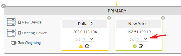
The device “weight” select menu shown at the far right of your server or device within a Server Group allows you to adjust how traffic is distributed by the load balancer when you have two or more devices in a configuration. In essence, the higher the number, the heavier the weight, and the more traffic that device will receive. But it does get more complex than that, so in this article, we’ll explain exactly how to use this feature to manipulate traffic distribution by the load balancer.

When should weight be used?

There are a number of reasons you may want to weight your servers differently. Perhaps one has greater network capacity or more horsepower, or perhaps it is at a primary data center location that is more central to your user base. Whatever the reason, it should be noted that all weight settings will deliver traffic to a device at some point. Weight is not a substitute for configuring a Failover Group if you truly need a device to be completely passive until all active devices go down. In other words, you cannot give your active server(s) a weight of 99 and your passive server(s) a weight of 1 and assume the servers with a weight of 1 will not receive any traffic. Servers with a weight of 1 in this type of configuration will still receive a small amount of traffic, and if this is undesirable, should not be used in place of failover.

When is weight taken into consideration?

First, it is important to note that the weight value can only impact load balancing traffic where one of these load balancing methods is used:

• Least Connection
• Round Robin
• Least Response Time
• Least Bandwidth
• Least Packets

If using a hash-type load balancing method, the weight is disregarded. When using a supported load balancing method as listed above, the load balancer will favor a device with the best combination of the fewest connections/active transactions/best response time/least bandwidth AND the highest weight using a computed Real Weight (rW) value.

It is important to note, however, that this plays out effectively when there is actual traffic on the load balancer (e.g. more than 1 active connection per server). We often find customers testing this with little to no traffic, perhaps only the test traffic they are generating. In a situation like this, where the devices / servers have no traffic or active transactions, new connections are sent to them in a round-robin fashion, because all things are considered equal at that point. Until the servers are loaded with 1 connection each, a computed Real Weight is not used and round-robin remains in effect. For example, if you have 3 servers and only 2 have connections, it does not matter how low the weight is for the server that does not yet have a connection. It will still receive the next connection because it has zero and the other two have one connection.

Additionally, it is important to note that if all devices / servers have the same weight, traffic will be distributed equally. In such a configuration, it is irrelevant what the weight value is. If all servers have a weight of 1 or all servers have a weight of 100, all things are equal and traffic is distributed equally.

How the Real Weight (rW) is computed when using the Least Connection method

Beyond the very first connection to each server, which is sent round-robin as we outlined above, a Real Weight (rW) is computed based on the Set Weight (sW) you give the device in the cloud management portal as well as the current number of active connections using the following formula:

Real Weight (rW) = Number of Active Connections x (10000 / Set Weight (sW))

After computation using the formula above, the lowest Real Weight (rW) is used to identify the server that will receive the next connection.

Clear as mud, right? Perhaps we should demonstrate.

A real example of weight utilization

Here is an example that may help to clarify how the weight impacts load balancing by using the least connection method. Let’s assume we have 3 servers, and they have been given the following Set Weight (sW):

• Server A – sW = 2
• Server B – sW = 3
• Server C – sW = 4

Based on the formula given above, before any connections are seen, the servers have this Real Weight (rW):

• Server A – rW = # connections x (10000 / sW) which is 0 x (10000/2) = 0
• Server B – rW = # connections x (10000 / sW) which is 0 x (10000/3) = 0
• Server C – rW = # connections x (10000 / sW) which is 0 x (10000/4) = 0

So, obviously all things are equal for the first connection, and all servers will be loaded up with 1 connection using round-robin before any further connections are given. This would be a total of 3 connections to load these servers up. And, of course, for the purposes of this article, we’ll assume these connections are persistent.

But the 4^th connection now invokes the computed rW, it results in the following:

• Server A – rW = 1 x 5000 = 5000
• Server B – rW = 1 x 3333 = 3333
• Server C – rW = 1 x 2500 = 2500

So the 4^th connection goes to Server C because it has the lowest rW.

Let’s figure out which server gets the 5^th connection

• Server A – rW = 1 x 5000 = 5000
• Server B – rW = 1 x 3333 = 3333
• Server C – rW = 2 x 2500 = 5000

So the 5^th connection goes to Server B because it has the lowest rW.

Let’s do one more. Where does the 6^th connection go?

• Server A – rW = 1 x 5000 = 5000
• Server B – rW = 2 x 3333 = 6666
• Server C – rW = 2 x 2500 = 5000

Okay, in this situation, both Server A and Server C have an equal real weight, so the connection could go to either of them. The load balancer uses round robin to make that decision, and we might assume it will go to Server A, at least for this example.

So at this point, with only 6 connections, it is obvious that the weighting is difficult to see because it is quite likely that all 3 servers have 2 connections each at this point. So to show how this really starts to play out as more and more connections are added, let’s expand this to show you how the first 30 connections are distributed to the servers, again, assuming they persist.

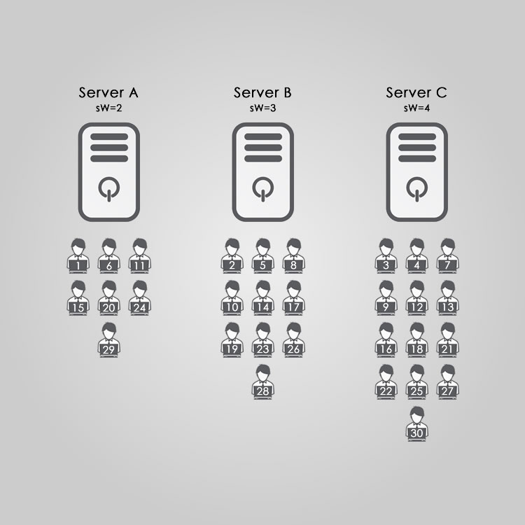
In the diagram above, each numbered person icon represents the connection, in the order they are created and distributed. And with 30 active connections, you can now see that Server C is definitely getting more traffic than Server B or Server A, as it should based on the different weights.

With weight options from 1 to 99 available in the cloud management portal, you might wonder how this would play out if we changed the server weighting to reflect a greater difference between the servers? Perhaps something like this?

• Server A – sW = 1 – giving it a rW of 10000
• Server B – sW = 50 – giving it a rW of 200
• Server C – sW = 99 – giving it a rW of 101

Here is a revised chart showing how the first 30 connections are now distributed to the servers based on their new weights.

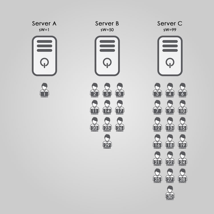
Now you can clearly see how the different weighting plays out in this example. Of course, these examples assume that once a connection is made, it persists, as I mentioned above. But with something as common and short-lived as HTTP traffic, when the connection is closed, everything is recomputed based on the current connections at that time, so this example does simplify it.

In the case of Server A in this latest example and diagram, assuming all connections remained active, it would not receive another connection until Server C reached 100 connections. But if the active connection on Server A ended, it would receive the very next connection because it then had 0 and round-robin would come into play.

Of course, these examples were for the Least Connection load balancing method. This plays out in a somewhat similar way for Round Robin because it is merely counting number of connections distributed vs. active. Least Bandwidth and Least Packets, however, change the formula so it is no longer the number of connections x (10000 / sW) but rather the current byte rate/second or current packets/second. This could drastically change things if, for example, one client was using an HTTP connection to download a large file, where another was merely loading small website objects. But it will work in a similar desired fashion to ensure that the server with the highest weight, receives the most traffic without fail. It is just a reminder that changing the load balancing method may require fine tuning of the weights.

We hope that this article has been helpful. If you have any questions, please reach out to us! We’re here to help you 24x7x365 whether you are a paying customer, or evaluating our solution on a free trial.